Friedman 1 model
We consider a modified version of the Friedman 1 dataset Friedman [Fri91] to examine the performance of our adaptive annealing scheduler in a high-dimensional context. According to the original model in Friedman [Fri91], the data are generated as
where \(\epsilon_i\sim\mathcal{N}(0,1)\). We made a slight modification to the model in (5) as
and set the true parameter combination to \(\boldsymbol{\beta}=(\beta_1,\ldots,\beta_{10})=(10,\pm \sqrt{20}, 0.5, 10, 5, 0, 0, 0, 0, 0)\). Note that both (5) and (6) contain linear, non-linear, and interaction terms of the input variables \(X_1\) to \(X_{10}\), five of which (\(X_6\) to \(X_{10}\)) are irrelevant to \(Y\). Each \(X\) is drawn independently from \(\mathcal{U}(0,1)\). We used R package tgp Gramacy [Gra07] to generate a Friedman 1 dataset with a sample size of \(n=1000\).
We impose a non-informative uniform prior \(p(\boldsymbol{\beta})\) and, unlike the original modal, we now expect a bimodal posterior distribution of \(\boldsymbol{\beta}\). Results in terms of marginal statistics and their convergence for the mode with positive \(z_{K,2}\) are illustrated in Table 1 and Fig. 5.
Exact |
Posterior Mean |
Posterior SD |
|---|---|---|
\(\beta_1 = 10\) |
10.0285 |
0.1000 |
\(\beta_2 = \pm \sqrt{20}\) |
4.2187 |
0.1719 |
\(\beta_3 = 0.5\) |
0.4854 |
0.0004 |
\(\beta_4 = 10\) |
10.0987 |
0.0491 |
\(\beta_5 = 5\) |
5.0182 |
0.1142 |
\(\beta_6 = 0\) |
0.1113 |
0.0785 |
\(\beta_7 = 0\) |
0.0707 |
0.0043 |
\(\beta_8 = 0\) |
-0.1315 |
0.1008 |
\(\beta_9 = 0\) |
0.0976 |
0.0387 |
\(\beta_{10} = 0\) |
0.1192 |
0.0463 |
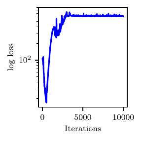
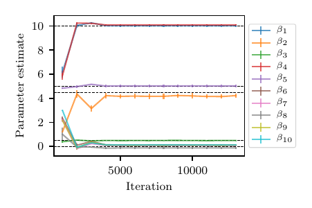
Fig. 5 Loss profile (left) and posterior marginal statistics for positive mode in the modified Friedman test case.
An implementation of this model can be found below.
    def adaann_example(self):

        # Quick run when repository is pushed
        if "it" in os.environ:
          run_T_1  = int(os.environ["it"])
          run_T    = 1
          run_T_0  = 1
          run_t0   = 0.99
        else:
          run_T_1  = 10000
          run_T    = 3
          run_T_0  = 500
          run_t0   = 0.001

        print('')
        print('--- TEST 5: FRIEDMAN 1 MODEL - ADAANN')
        print('')

        from linfa.run_experiment import experiment

        # Experiment Setting
        exp = experiment()
        exp.name              = "adaann"
        exp.flow_type         = 'realnvp'     # str: Type of flow (default 'realnvp')
        exp.n_blocks          = 10            # int: Number of layers (default 5)
        exp.hidden_size       = 20            # int: Hidden layer size for MADE in each layer (default 100)
        exp.n_hidden          = 1             # int: Number of hidden layers in each MADE (default 1)
        exp.activation_fn     = 'relu'        # str: Actication function used (default 'relu')
        exp.input_order       = 'sequential'  # str: Input order for create_mask (default 'sequential')
        exp.batch_norm_order  = True          # bool: Order to decide if batch_norm is used (default True)
        exp.save_interval     = 1000          # int: How often to sample from normalizing flow

        exp.input_size   = 10     # int: Dimensionality of input (default 2)
        exp.batch_size   = 100    # int: Number of samples generated (default 100)
        exp.lr           = 0.005  # float: Learning rate (default 0.003)
        # exp.lr_decay   = 0.75
        exp.lr_decay     = 0.9
        exp.log_interval = 10     # int: How often to show loss stat (default 10)
        exp.run_nofas    = False
        exp.annealing    = True

        exp.optimizer    = 'Adam'    # str: type of optimizer used
        exp.lr_scheduler = 'StepLR'  # str: type of lr scheduler used
        exp.lr_step      = 500       # int: number of steps for lr step scheduler
        exp.tol          = 0.4       # float: tolerance for AdaAnn scheduler
        # exp.t0           = 0.001     # float: initial inverse temperature value
        exp.t0           = run_t0
        exp.N            = 100       # int: number of sample points during annealing
        exp.N_1          = 400       # int: number of sample points at t=1
        # exp.T_0          = 500       # int: number of parameter updates at initial t0
        # exp.T            = 3         # int: number of parameter updates during annealing
        # exp.T_1          = 10000     # int: number of parameter updates at t=1
        exp.T_0          = run_T_0
        exp.T            = run_T
        exp.T_1          = run_T_1
        exp.M            = 1000      # int: number of sample points used to update temperature
        exp.scheduler    = 'AdaAnn'  # str: type of annealing scheduler used

        exp.output_dir   = './results/' + exp.name
        exp.log_file     = 'log.txt'
        # exp.seed = 35435  # int: Random seed used
        exp.seed         = random.randint(0, 10 ** 9)  # int: Random seed used
        exp.n_sample     = 5000                        # int: Batch size to generate final results/plots
        exp.no_cuda      = True                        # Running on CPU by default but tested on CUDA

        exp.device = torch.device('cuda:0' if torch.cuda.is_available() and not exp.no_cuda else 'cpu')

        # Model Setting
        res_path = os.path.abspath(os.path.join(os.path.dirname(linfa.__file__), os.pardir))
        data_set = np.loadtxt(res_path + '/resource/data/D1000.csv',delimiter=',',skiprows=1)
        data = torch.tensor(data_set).to(exp.device)

        def log_density(params, d):

            # Compute Model
            # Modified bimodal version of the Friedman model
            def targetPosterior(b, x):
                return b[0] * torch.sin(np.pi * x[:, 0] * x[:, 1]) + \
                       (b[1] ** 2) * (x[:, 2] - b[2]) ** 2 + \
                       x[:, 3] * b[3] + \
                       x[:, 4] * b[4] + \
                       x[:, 5] * b[5] + \
                       x[:, 6] * b[6] + \
                       x[:, 7] * b[7] + \
                       x[:, 8] * b[8] + \
                       x[:, 9] * b[9]

            f = torch.zeros(len(params)).to(exp.device)

            for i in range(len(params)):
                y_out = targetPosterior(params[i], d)
                val = torch.linalg.norm(y_out - d[:, 10])
                f[i] = -val ** 2 / 2

            return f

        exp.model_logdensity = lambda x: log_density(x, data)
        exp.run()