Three-element Wndkessel Model
The three-parameter Windkessel or RCR model is characterized by proximal and distal resistance parameters \(R_{p}, R_{d} \in [100, 1500]\) Barye \(\cdot\) s/ml and one capacitance parameter \(C \in [1\times 10^{-5}, 1\times 10^{-2}]\) ml/Barye.
This model is not identifiable. The average distal pressure is only affected by the total system resistance, i.e. the sum \(R_{p}+R_{d}\), leading to a negative correlation between these two parameters. Thus, an increment in the proximal resistance is compensated by a reduction in the distal resistance (so the average distal pressure remains the same) which, in turn, reduces the friction encountered by the flow exiting the capacitor. An increase in the value of \(C\) is finally needed to restore the average, minimum and maximum pressure. This leads to a positive correlation between \(C\) and \(R_{d}\).
The output consists of the maximum, minimum and average values of the proximal pressure \(P_{p}(t)\), i.e., \((P_{p,\text{min}}, P_{p,\text{max}}, P_{p,\text{avg}})\) over one heart cycle. The true parameters are \(z^{*}_{K,1} = R^{*}_{p} = 1000\) Barye \(\cdot\) s/ml, \(z^{*}_{K,2}=R^{*}_{d} = 1000\) Barye \(\cdot\) s/ml and \(C^{*} = 5\times 10^{-5}\) ml/Barye and the proximal pressure is computed from the solution of the algebraic-differential system
where the distal pressure is set to \(P_{d}=55\) mmHg.
Synthetic observations are generated from \(N(\boldsymbol\mu, \boldsymbol\Sigma)\), where \(\mu=(f_{1}(\boldsymbol{z}^{*}),f_{2}(\boldsymbol{z}^{*}),f_{3}(\boldsymbol{z}^{*}))^T = (P_{p,\text{min}}, P_{p,\text{max}}, P_{p,\text{ave}})^T = (100.96, 148.02,116.50)^T\) and \(\boldsymbol\Sigma\) is a diagonal matrix with entries \((5.05, 7.40, 5.83)^T\). The budgeted number of true model solutions is 216; the fixed surrogate model is evaluated on a \(6\times 6\times 6 = 216\) pre-grid while the adaptive surrogate is evaluated with a pre-grid of size \(4\times 4\times 4 = 64\) and the other 152 evaluations are adaptively selected.
This example also demonstrates how NoFAS can be combined with annealing for improved convergence. The results in Fig. 4 are generated using the AdaAnn adaptive annealing scheduler with intial inverse temperature \(t_{0}=0.05\), KL tolerance \(\tau=0.01\) and a batch size of 100 samples. The number of parameter updates is set to 500, 5000 and 5 for \(t_{0}\), \(t_{1}\) and \(t_{0}<t<t_{1}\), respectively and 1000 Monte Carlo realizations are used to evaluate the denominator in (5). Use of annealing explains why the loss function is increasing (the posterior distribution becomes increasingly less smooth) instead of monotonically descreasing as for the other examples. The posterior samples capture well the nonlinear correlation among the parameters and generate a fairly accurate posterior predictive distribution that overlaps with the observations. Additional details can be found in [CHLS23, WLS22].
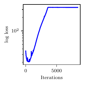
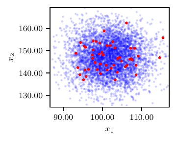
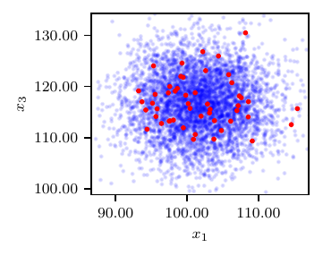
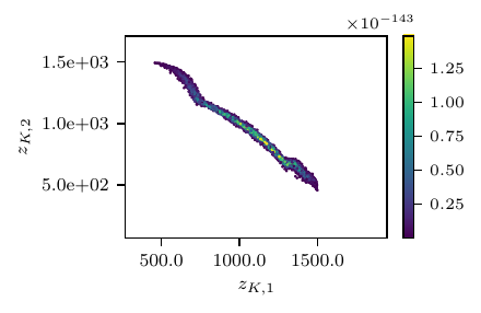
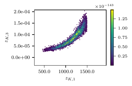
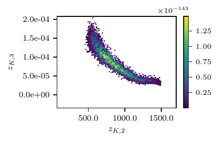
Fig. 4 Results from the RCR model. Loss profile (top), posterior predictive distribution (center) and posterior samples (bottom).
An implementation of this model can be found below.
    def rcr_example(self):

        if "it" in os.environ:
          max_it  = int(os.environ["it"])
          max_pre = 1000
        else:
          max_it  = 25001
          max_pre = 50000

        print('')
        print('--- TEST 4: RCR MODEL - NOFAS')
        print('')

        # Import rcr model
        from linfa.models.circuit_models import rcrModel

        exp = experiment()
        exp.name = "rcr"
        exp.flow_type         = 'maf'         # str: Type of flow (default 'realnvp')
        exp.n_blocks          = 15            # int: Number of layers (default 5)
        exp.hidden_size       = 100           # int: Hidden layer size for MADE in each layer (default 100)
        exp.n_hidden          = 1             # int: Number of hidden layers in each MADE (default 1)
        exp.activation_fn     = 'relu'        # str: Actication function used (default 'relu')
        exp.input_order       = 'sequential'  # str: Input order for create_mask (default 'sequential')
        exp.batch_norm_order  = True          # bool: Order to decide if batch_norm is used (default True)
        exp.save_interval = 5000          # int: How often to sample from normalizing flow

        exp.input_size    = 3       # int: Dimensionality of input (default 2)
        exp.batch_size    = 500     # int: Number of samples generated (default 100)
        exp.true_data_num = 2       # double: number of true model evaluated (default 2)
        # exp.n_iter        = 25001   # int: Number of iterations (default 25001)
        exp.n_iter        = max_it
        exp.lr            = 0.003   # float: Learning rate (default 0.003)
        exp.lr_decay      = 0.9999  # float: Learning rate decay (default 0.9999)
        exp.log_interval  = 10      # int: How often to show loss stat (default 10)

        exp.run_nofas          = True
        exp.surr_pre_it       = max_pre #:int: Number of pre-training iterations for surrogate model
        exp.surr_upd_it       = 6000  #:int: Number of iterations for the surrogate model update

        exp.annealing          = False
        exp.calibrate_interval = 300  # int: How often to update surrogate model (default 1000)
        exp.budget             = 216  # int: Total number of true model evaluation
        exp.surr_folder        = "./"
        exp.use_new_surr       = True

        exp.output_dir = './results/' + exp.name
        exp.log_file = 'log.txt'
        exp.seed = random.randint(0, 10 ** 9)  # int: Random seed used
        exp.n_sample = 5000                    # int: Batch size to generate final results/plots
        exp.no_cuda = True                     # Running on CPU by default but tested on CUDA

        exp.optimizer = 'RMSprop'
        exp.lr_scheduler = 'ExponentialLR'

        exp.device = torch.device('cuda:0' if torch.cuda.is_available() and not exp.no_cuda else 'cpu')

        # Define transformation
        # One list for each variable
        trsf_info = [['tanh',-7.0,7.0,100.0,1500.0],
                     ['tanh',-7.0,7.0,100.0,1500.0],
                     ['exp',-7.0,7.0,1.0e-5,1.0e-2]]
        trsf = Transformation(trsf_info)
        exp.transform = trsf

        # Define model
        cycleTime = 1.07
        totalCycles = 10
        res_path = os.path.abspath(os.path.join(os.path.dirname(linfa.__file__), os.pardir))
        forcing = np.loadtxt(res_path + '/resource/data/inlet.flow')
        model = rcrModel(cycleTime, totalCycles, forcing, device=exp.device)  # RCR Model Defined
        exp.model = model

        # Read data
        model.data = np.loadtxt(res_path + '/resource/data/data_rcr.txt')

        # Define surrogate
        exp.surrogate = Surrogate(exp.name, lambda x: model.solve_t(trsf.forward(x)), exp.input_size, 3,
                                  model_folder=exp.surr_folder, limits=torch.Tensor([[-7, 7], [-7, 7], [-7, 7]]),
                                  memory_len=20, device=exp.device)
        surr_filename = exp.surr_folder + exp.name
        if exp.use_new_surr or (not os.path.isfile(surr_filename + ".sur")) or (not os.path.isfile(surr_filename + ".npz")):
            print("Warning: Surrogate model files: {0}.npz and {0}.npz could not be found. ".format(surr_filename))
            exp.surrogate.gen_grid(gridnum=4)
            exp.surrogate.pre_train(exp.surr_pre_it, 0.03, 0.9999, 500, store=True)
        # Load the surrogate
        exp.surrogate.surrogate_load()

        # Define log density
        def log_density(x, model, surrogate, transform):

            # Compute transformation log Jacobian
            adjust = transform.compute_log_jacob_func(x)

            if surrogate:
                modelOut = surrogate.forward(x)
            else:
                modelOut = model.solve_t(transform.forward(x))

            # Get the absolute values of the standard deviations
            stds = model.defOut * model.stdRatio
            Data = torch.tensor(model.data).to(exp.device)

            # Eval LL
            ll1 = -0.5 * np.prod(model.data.shape) * np.log(2.0 * np.pi)  # a number
            ll2 = (-0.5 * model.data.shape[1] * torch.log(torch.prod(stds))).item()  # a number
            ll3 = 0.0
            for i in range(3):
                ll3 += - 0.5 * torch.sum(((modelOut[:, i].unsqueeze(1) - Data[i, :].unsqueeze(0)) / stds[0, i]) ** 2, dim=1)
            negLL = -(ll1 + ll2 + ll3)
            res = -negLL.reshape(x.size(0), 1) + adjust

            # Return LL
            return res

        # Assign logdensity model
        exp.model_logdensity = lambda x: log_density(x, model, exp.surrogate, trsf)

        # Run VI
        exp.run()