Two-element Windkessel Model
The two-element Windkessel model (often referred to as the RC model) is the simplest representation of the human systemic circulation and requires two parameters, i.e., a resistance \(R \in [100, 1500]\) Barye \(\cdot\) s/ml and a capacitance \(C \in [1\times 10^{-5}, 1 \times 10^{-2}]\) ml/Barye.
We provide a periodic time history of the aortic flow (see [WLS22] for additional details) and use the RC model to predict the time history of the proximal pressure \(P_{p}(t)\), specifically its maximum, minimum and average values over a typical heart cycle, while assuming the distal resistance \(P_{d}(t)\) as a constant in time, equal to 55 mmHg.
In our experiment, we set the true resistance and capacitance as \(z_{K,1}^{*}=R^{*} = 1000\) Barye:math:cdot s/ml and \(z_{K,2}^{*}=C^{*} = 5\times 10^{-5}\) ml/Barye and determine \(P_{p}(t)\) from a RK4 numerical solution of the following algebraic-differential system
where \(Q_{p}\) is the flow entering the RC system and \(Q_{d}\) is the distal flow.
Synthetic observations are generated by adding Gaussian noise to the true model solution \(\boldsymbol{x}^{*}=(x^{*}_{1},x^{*}_{2},x^{*}_{3})=(P_{p,\text{min}},\) \(P_{p,\text{max}},\) \(P_{p,\text{avg}})= (78.28, 101.12, 85.75)\), i.e., \(\boldsymbol{x}\) follows a multivariate Gaussian distribution with mean \(\boldsymbol{x}^{*}\) and a diagonal covariance matrix with entries \(0.05\,x_{i}^{*}\), where \(i=1,2,3\) corresponds to the maximum, minimum, and average pressures, respectively.
The aim is to quantify the uncertainty in the RC model parameters given 50 repeated pressure measurements. We imposed a non-informative prior on \(R\) and \(C\). Results are shown in Fig. 3.
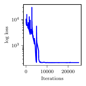
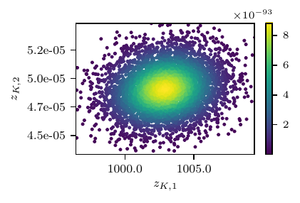
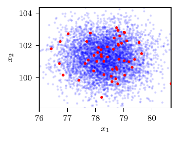
Fig. 3 Results from the RC model. Loss profile (top), posterior samples (center) for R and C and the posterior predictive distribution (bottom) for \(P_{p,\text{min}}\) and \(P_{p,\text{max}}\) (right, \(P_{p,\text{avg}}\) not shown).
An implementation of this model can be found below.
    def rc_example(self):

        if "it" in os.environ:
          max_it  = int(os.environ["it"])
          max_pre = 1000
        else:
          max_it  = 25001
          max_pre = 40000

        print('')
        print('--- TEST 3: RC MODEL - NOFAS')
        print('')

        # Import model
        from linfa.models.circuit_models import rcModel

        exp = experiment()
        exp.name = "rc"
        exp.flow_type         = 'maf'         # str: Type of flow (default 'realnvp')
        exp.n_blocks          = 5             # int: Number of layers (default 5)
        exp.hidden_size       = 100           # int: Hidden layer size for MADE in each layer (default 100)
        exp.n_hidden          = 1             # int: Number of hidden layers in each MADE (default 1)
        exp.activation_fn     = 'relu'        # str: Actication function used (default 'relu')
        exp.input_order       = 'sequential'  # str: Input order for create_mask (default 'sequential')
        exp.batch_norm_order  = True          # bool: Order to decide if batch_norm is used (default True)
        exp.save_interval = 5000          # int: How often to sample from normalizing flow

        exp.input_size    = 2       # int: Dimensionality of input (default 2)
        exp.batch_size    = 250     # int: Number of samples generated (default 100)
        exp.true_data_num = 2       # int: number of true model evaluated (default 2)
        # exp.n_iter        = 25001   # int: Number of iterations (default 25001)
        exp.n_iter        = max_it
        exp.lr            = 0.005   # float: Learning rate (default 0.003)
        exp.lr_decay      = 0.9999  # float: Learning rate decay (default 0.9999)
        exp.log_interval  = 10      # int: How often to show loss stat (default 10)

        exp.run_nofas          = True
        exp.surr_pre_it       = max_pre #:int: Number of pre-training iterations for surrogate model
        exp.surr_upd_it       = 6000  #:int: Number of iterations for the surrogate model update

        exp.annealing          = False
        exp.calibrate_interval = 1000  # int: How often to update surrogate model (default 1000)
        exp.budget             = 64    # int: Total number of true model evaluation
        exp.surr_folder        = "./"
        exp.use_new_surr       = True

        exp.output_dir   = './results/' + exp.name
        exp.log_file     = 'log.txt'
        exp.seed         = random.randint(0, 10 ** 9)  # int: Random seed used
        exp.n_sample     = 5000                        # int: Batch size to generate final results/plots
        exp.no_cuda      = True                        # Running on CPU by default but tested on CUDA

        exp.optimizer = 'RMSprop'
        exp.lr_scheduler = 'ExponentialLR'

        exp.device = torch.device('cuda:0' if torch.cuda.is_available() and not exp.no_cuda else 'cpu')

        # Define transformation
        # One list for each variable
        trsf_info = [['tanh',-7.0,7.0,100.0,1500.0],
                     ['exp',-7.0,7.0,1.0e-5,1.0e-2]]
        trsf = Transformation(trsf_info)
        exp.transform = trsf

        # Define model
        cycleTime = 1.07
        totalCycles = 10
        res_path = os.path.abspath(os.path.join(os.path.dirname(linfa.__file__), os.pardir))
        forcing = np.loadtxt(res_path + '/resource/data/inlet.flow')
        model = rcModel(cycleTime, totalCycles, forcing, device=exp.device)  # RCR Model Defined
        exp.model = model

        # Read Data
        model.data = np.loadtxt(res_path + '/resource/data/data_rc.txt')

        # Define surrogate model
        exp.surrogate = Surrogate(exp.name, lambda x: model.solve_t(trsf.forward(x)), exp.input_size, 3,
                                  model_folder=exp.surr_folder, limits=torch.Tensor([[-7, 7], [-7, 7]]),
                                  memory_len=20, device=exp.device)
        surr_filename = exp.surr_folder + exp.name
        if exp.use_new_surr or (not os.path.isfile(surr_filename + ".sur")) or (not os.path.isfile(surr_filename + ".npz")):
            print("Warning: Surrogate model files: {0}.npz and {0}.npz could not be found. ".format(surr_filename))
            exp.surrogate.gen_grid(gridnum=4)
            exp.surrogate.pre_train(exp.surr_pre_it, 0.03, 0.9999, 500, store=True)
        # Load the surrogate
        exp.surrogate.surrogate_load()

        # Define log density
        def log_density(x, model, surrogate, transform):

            # Compute transformation log Jacobian
            adjust = transform.compute_log_jacob_func(x)

            if surrogate:
                modelOut = surrogate.forward(x)
            else:
                modelOut = model.solve_t(transform.forward(x))

            # Get the absolute values of the standard deviations
            stds = model.defOut * model.stdRatio
            Data = torch.tensor(model.data).to(exp.device)

            # Eval Gaussian LL
            ll1 = -0.5 * np.prod(model.data.shape) * np.log(2.0 * np.pi)  # a number
            ll2 = (-0.5 * model.data.shape[1] * torch.log(torch.prod(stds))).item()  # a number
            ll3 = 0.0
            for i in range(3):
                ll3 += - 0.5 * torch.sum(((modelOut[:, i].unsqueeze(1) - Data[i, :].unsqueeze(0)) / stds[0, i]) ** 2, dim=1)
            negLL = -(ll1 + ll2 + ll3)
            res = -negLL.reshape(x.size(0), 1) + adjust

            # Return LL
            return res

        # Assign log-density
        exp.model_logdensity = lambda x: log_density(x, model, exp.surrogate, trsf)

        # Run VI
        exp.run()